Python Data Analysis With Sqlite And Pandas
As a step in me learning Data Analysis With Python I wanted to
- set up a database
- write values to it (to fake statistics from production)
- read values from the database into pandas
- do some filtering with pandas
- make a plot with matplotlib.
So this text describes these steps.
Set up the environment
To spice things up I wanted this to run on a raspberry pi (see Dagbok 20151215). I started with the Raspbian Lite image from the official Raspberry pi downloads page (see [1]).
This was a fun but painfully slow way to set up the environment. I should probably have spend twice as much on the micro-SD card to get it faster if I had known this. I also first used Wifi instead of a wired ethernet connection.
After running sudo raspi-config to make use of the entire storage I made an update and installed my favorite desktop environment (Xfce), a nice editor (Gnu Emacs) and the python packages I needed:
sudo apt-get update
sudo apt-get upgrade
sudo apt-get install emacs-nox
sudo apt-get install xfce4 xfce4-goodies xfce4-screenshooter
sudo apt-get install sqlite3
sudo apt-get install python-scipy
sudo apt-get install python-pandas
sudo apt-get install ...
Set up the database
I wanted to use some form of SQL database, and sqlite is perfect for the job. Since I want to do this programmatically I go through python. In this short example I connect to a (new) database and create a table called sensor.
conn = sqlite3.connect(FILENAME)
cur = conn.cursor()

sql = """
    create table sensor (
        sid         integer primary key not null,
        name        text,
        notes       text
    );"""

_ = cur.execute(sql)
I fill this and the other tables with some values. In fact I do this in a very complicated way just for fun and it turned out to be very, very slow. If you feel like getting the details scroll down and read the code in the full example.
sql = "insert into sensor(sid, name, notes) values (%d, '%s', '%s');"
for (uid, name, notes) in [(201, 'Alpha', 'Sensor for weight'), \
                           (202, 'Beta', 'Sensor for conductivity'),
                           (203, 'Gamma', 'Sensor for surface oxides'),
                           (204, 'Delta', 'Sensor for length'),
                           (205, 'Epsilon', 'Sensor for x-ray'),
                           (206, 'Zeta', 'Color checker 9000'),
                           (207, 'Eta', 'Ultra-violet detector'), ]:
    cur.execute(sql % (uid, name, notes))
The full example build this table, a few others and adds some 700 thousand faked sensor readings to the database. On my Raspberry Pi 2 this requires almost 6 minutes, but that's OK since it is intended to fake 7 years of sensor readings:
$ time python build.py
create new file /tmp/database.data
insert values from line 1

[...]

real	5m42.281s
user	5m6.020s
sys	0m11.460s
Read values from the database
We want to read the values and I experimented with sqlite default settings in my .sqliterc file. I tried this:
$ cat ~/.sqliterc
.mode column
.headers on
Anyway, I first try to do some database queries with the command line tool. If you have never used these before, I can only urge you to learn hand-crafting sql queries. It really speeds up debugging and experimentation to have a command line session running in parallel with the code being written. Here is a typical small session:
$ sqlite3 database.data

sqlite> select * from line;
lid         name        notes
----------  ----------  -----------------------------
101         L1          refurbished soviet line, 1956
102         L2          multi-purpose line from 1999
103         L3          mil-spec line, primary
104         L4          mil-spec line, seconday
As we saw above, when we created the values, communicating through python is super-easy, so now we want these values to go into pandas for data-analysis. As it turns out: this was also very easy once you figure out how. The tricky part was to figure out that the command I needed was pandas.read_sql(query, conn). This example works fine using IPython (see Ipython First Look), to use the syntax completion features, but it also works in a regular python session, or as a script:
import pandas
import matplotlib.pyplot as plt
import sqlite3

conn = sqlite3.connect('./database.data')

limit = 1000000
query = """
        select
            reading.rid, reading.timestamp, product.name as product,
            serial, line.name as line, sensor.name sensor, verdict
        from
            reading, product, line, sensor
        where
            reading.sid = sensor.sid and
            reading.pid = product.pid and
            reading.lid = line.lid
        limit %s;
        """ % limit

data = pandas.read_sql(query, conn)
We now have very many values in the data structure called data. My poor raspberry pi leaped from 225 MB of used memory to 465 MB, after peaking at more than 500 MB. Remember that this poor computer only has about 925 MB after giving some of it to the GPU.
Let's try to take a look at it by counting the values based on what line and product they represent:
print data.groupby(['line', 'product']).size()

line  product
L1    PA         183364
L2    PA          47247
      PB          57258
      PC         375084
L3    PB           7971
      PC          13311
L4    PD           1389
For someone who has not studied my toy example this means that on for example Line 3 we have recorder 7971 sensor readings on product of type PB and 13311 readings on products of type PC. These values are of course totally irrelevant, but imagine them being real values from a real raspberry pi project in a production site where you are responsible for improving the quality of the physical entities being produced. Then these values might mean that Line 4 is not living up to expectation and could be scrapped, or that product PB on Line L3 should instead be produced on line 4.
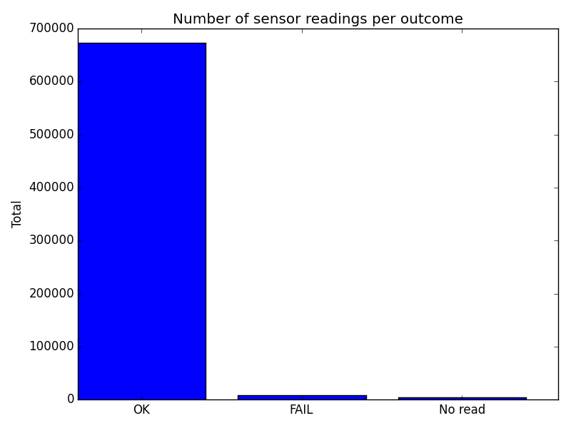
Make a plot
I made a bar-chart. But am not too happy with this example, I think the code is too verbose and bulky for a minimal example. Perhaps you can make it prettier. This nicely illustrates the power of scipy.
fig, ax = plt.subplots()
new_set = data.groupby('verdict').size()
width = 0.8
ax.bar([1,2,3], new_set, width=width)
plt.ylabel('Total')
plt.title('Number of sensor readings per outcome')
plt.xticks([1 + width/2, 2+ width/2,3+ width/2],
           ('OK', 'FAIL', 'No read'))

plt.tight_layout()
plt.savefig('python-data-analysis-sqlite-pandas.png')
And here is the plot, as created on a Raspberry Pi:
Summary
Data Analysis With Python is extremely powerful and can be done, with some pain, even on a raspberry pi. Download the full example from here: [2]
My next step is to pretend that the database solution does not scale to the new needs (all the new lines), so a front-end for presenting sensor readings and manually commenting on bad verdicts should be possible. We let this database be a legacy database and use Django: Python Data Presentation With Django And Legacy Sqlite Database
This page belongs in Kategori Programmering
See also Data Analysis With Python